Computational Pathology: Teaching Machines to Read Tissue

Introduction

Anyone who has sat across a double-headed microscope from an experienced pathologist knows the moment. A sweep at low power, a pause, a flick to high power on one cluster of cells, and a decision. Years of pattern recognition get compressed into a few seconds, and it is natural to wonder how much of that a machine could learn.

I came to pathology from the other direction. My PhD was in RNA biology and cardiovascular science: mouse models, sequencing, and molecular mechanisms, which I describe on my RNA biology page. In medical school I kept being drawn back to the place where all that molecular detail becomes a diagnosis, and that place is usually a glass slide. Clinical work in pathology, including hematopathology at Ohio State and a visiting clerkship at Brigham and Women’s and Mass General, and time spent annotating whole-slide images for computational pathology research, made me want to understand how this field fits together.

Computational pathology sits at an unusual intersection. The data are among the largest images in medicine, gigapixels per slide. The labels are expensive, noisy, and sometimes disputed by experts. The stakes are high: a pathology report often is the diagnosis, the thing that decides whether someone gets surgery, chemotherapy, or reassurance. And the field has moved fast, from hand-crafted nuclear measurements to deep networks to self-supervised foundation models trained on millions of slides, all in about fifteen years.

This page is a guide to that history and to where I think the field is now. It’s written for clinicians curious about AI, for machine-learning people curious about pathology, and for students deciding whether to work on this. Throughout, At the microscope boxes connect a topic to what actually happens at sign-out.

Start here: a viewing path

These are the videos I’d recommend, in order. The first three are the best visual introductions to the machine-learning ideas this page relies on.

1. But what is a neural network? (3Blue1Brown). The clearest twenty minutes on what a network is doing.
2. But what is a convolution? (3Blue1Brown). The operation at the heart of a decade of image models.
3. Attention in transformers, step by step (3Blue1Brown). The mechanism behind foundation models and vision–language models.
4. Validating whole slide imaging for digital pathology (Pathology Lens). What it takes to trust a scanned slide for diagnosis.
5. A.I.’s transformation of pathology (Faisal Mahmood with Eric Topol). A leading computational pathologist on foundation models and what’s next.
6. Multimodal, generative, and agentic AI for pathology (Faisal Mahmood, Broad Institute). A technical tour of the 2024–2025 frontier.

Part I: The Glass Slide (1858–1990)

Disease as a disorder of cells

In 1858 Rudolf Virchow published Cellular Pathology and argued that disease happens in cells. It sounds obvious now. At the time it made the microscope the center of diagnosis, and it set the basic workflow pathologists still follow: take tissue, fix it, cut it thin, stain it, and look.

The stain that won is hematoxylin and eosin, H&E, combined in the 1870s and still used on most diagnostic slides made today. Hematoxylin colors nuclei blue-purple; eosin colors cytoplasm and extracellular matrix shades of pink. Almost everything in this page, every algorithm and foundation model, is ultimately learning from those two dyes. In the 1940s, Albert Coons and colleagues showed that antibodies could be tagged and used to label specific molecules in tissue, the ancestor of immunohistochemistry. That added a third color and turned the slide into a molecular readout.

Pattern recognition, codified

Much of pathology is pattern recognition made explicit. In 1966 Donald Gleason, a pathologist at the Minneapolis VA, described prostate cancer by its architectural patterns, from well-formed glands to sheets of cells (Gleason, 1966). The Gleason system, refined many times since, still drives prostate cancer treatment. Grading systems like it are a gift to machine learning: they are explicit, visual, and tied to outcomes.

They are also hard to apply consistently. That matters, because in machine learning, the pathologist’s diagnosis usually becomes the “ground truth” a model is trained to reproduce.

How often do pathologists agree?

In a large 2015 study, 115 U.S. pathologists each interpreted 60 breast biopsies, and their diagnoses were compared with an expert consensus (Elmore et al., 2015). Agreement was high for invasive cancer and fell sharply for the borderline category of atypical hyperplasia.

I don’t read this as a story about pathologists being unreliable. Most of the disagreement sits at diagnostic boundaries that are hard by nature, with real consequences in both directions. But it carries two lessons for computational pathology. A model trained on one pathologist’s labels learns that pathologist’s thresholds. And for borderline categories, the most useful thing an algorithm may offer is not a “correct” answer but a reproducible one.

The first computer vision in pathology

People were trying to automate this long before deep learning. In 1966, Judith Prewitt and Mortimer Mendelsohn published “The analysis of cell images”, a study that digitized images of blood cells and classified them by computed features (Prewitt & Mendelsohn, 1966). It is often cited as the beginning of the field. By the mid-1990s, automated systems for screening cervical Pap smears had reached the U.S. market, and automated blood-smear morphology analyzers followed in hematology labs. Those systems worked because the task was constrained: single cells on a flat preparation, with a clear abnormal-versus-normal question. Tissue sections, with their architecture, overlapping cells, and staining variation, would take another generation of technology.

Part II: Going Digital (1999–2020)

From microscope to scanner

A whole-slide scanner is a robotic microscope with a camera. It captures thousands of overlapping fields at high magnification and stitches them into one image, stored as a pyramid of resolutions so a viewer can zoom from the whole slide down to individual cells. At “40×”, a typical scan resolution, each pixel covers about a quarter of a micron. A tissue section a centimeter or two across becomes an image tens of thousands of pixels on a side.

It’s hard to get an intuition for the numbers, so here is a calculator. Change the tissue size, scan magnification, and tile size, and see what a model actually has to process.

Standards and regulation

Digitization needed plumbing. In 2010, the DICOM imaging standard used in radiology added a specification for whole-slide images, so slides could eventually live in the same systems as CT scans. In 2017, the FDA authorized a whole-slide imaging system for primary diagnosis in the U.S. for the first time. Pathologists could legally sign out cases from a screen. During the COVID-19 pandemic, emergency waivers let pathologists review cases remotely, and many departments that had been piloting digital workflows moved them into routine use.

Going digital is not trivial. Every lab has to validate that diagnoses made on screen match those made on glass, and some tasks, like spotting tiny organisms or judging subtle nuclear detail, can be harder on a monitor.

Part III: Hand-Crafted Features (2005–2014)

Measuring what pathologists see

The first wave of modern computational pathology tried to measure what pathologists describe. Segment the nuclei, then compute their size, shape, and texture; measure how glands are arranged; quantify the stroma. Feed hundreds of these engineered features into a classifier.

The most influential example was C-Path in 2011. Andrew Beck, Daphne Koller, and colleagues extracted thousands of features from breast cancer images and found that features of the stroma, the supporting tissue around tumor cells, predicted survival as well as or better than features of the cancer cells themselves (Beck et al., 2011). Pathologists hadn’t been grading the stroma. The algorithm suggested they had been overlooking prognostic information hiding in plain sight.

The problem of color

A problem appeared early and has never fully gone away: slides from different labs look different. Stain batches, staining time, section thickness, and scanner optics all shift color and texture. A model trained in one hospital can stumble in another. Researchers developed stain normalization methods that map every slide onto a reference color profile, and later augmentation strategies that randomly perturb color during training so models learn to ignore it. Part VIII returns to why this is still the field’s central problem.

Deep learning arrives through mitoses

Counting mitoses, cells caught in the act of dividing, is part of grading breast cancer. It’s tedious and variable, which made it a natural challenge problem. In the 2012 ICPR mitosis-detection contest, the winning entry was a deep convolutional network from Dan Cireşan, Jürgen Schmidhuber, and colleagues (Cireşan et al., 2013). That was the same year AlexNet won ImageNet. Deep learning came to pathology at almost exactly the moment it came to computer vision as a whole.

Part IV: Deep Learning Takes Over (2015–2019)

Convolutions on tissue

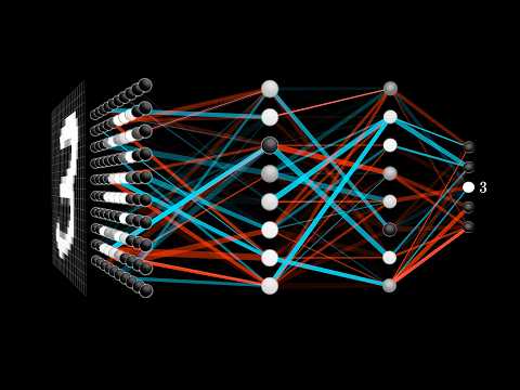
A convolutional neural network slides small learned filters across an image. Early layers learn edges and color blobs; deeper layers combine them into textures, nuclei, glands, and eventually patterns that predict a diagnosis. Crucially, nobody tells the network which features to compute. It learns them from labeled examples. That was the end of hand-crafted features.

U-Net and the art of drawing boundaries

Classifying a tile is one task. Outlining exactly where a tumor, a gland, or a nucleus is, segmentation, is another. In 2015, Olaf Ronneberger, Philipp Fischer, and Thomas Brox introduced U-Net, designed for biomedical images. It compresses an image through an encoder, expands it back through a decoder, and passes high-resolution detail across “skip connections” so the output map is sharp. U-Net and its descendants, including the nested UNet++, remain workhorses for segmentation in pathology. A common modern recipe pairs a U-Net-style decoder with a pretrained foundation-model encoder.

CAMELYON16: the moment that got attention

In 2016, a team led from Radboud University ran a challenge: detect breast cancer metastases in sentinel lymph node slides. Teams trained on 270 slides and were tested on 129 more. The same 129 slides were read by 11 pathologists in a timed session meant to simulate routine work, and by one pathologist with no time limit (Ehteshami Bejnordi et al., 2017).

The headline that “AI beat pathologists” was too simple. The task was narrow, the pathologists in the timed arm were rushed, and the unhurried pathologist was nearly as good as the machines. But it was a real demonstration that, for a well-defined detection task, deep learning could match expert performance on whole slides. It also showed where an algorithm earns its keep: finding a small cluster of metastatic cells in a large node is exactly the tedious search that fatigue makes hard for humans.

Morphology predicts molecules

Then came a stranger result. In 2018, Nicolas Coudray, Aristotelis Tsirigos, and colleagues trained a network on lung cancer slides from The Cancer Genome Atlas. It classified tumor subtypes, and it could also predict, better than chance, whether several commonly mutated genes, including EGFR, KRAS, and STK11, were mutated, from the H&E slide alone (Coudray et al., 2018). A year later, Jakob Kather and colleagues predicted microsatellite instability, a key determinant of immunotherapy eligibility, directly from H&E in gastrointestinal cancers (Kather et al., 2019).

These results connect directly to my RNA work. Genotype shapes gene expression, gene expression shapes cells, and cells shape the patterns a pathologist sees, so the slide carries a faint imprint of the molecular state. In 2020, a model called ST-Net predicted spatially resolved gene expression from H&E images, trained on spatial transcriptomics data (He et al., 2020), a technology that measures RNA in place across a tissue section (Ståhl et al., 2016).

Part V: The Slide Is a Bag of Tiles (2018–2021)

The labeling problem

CAMELYON needed pathologists to outline every metastasis by hand, which is painstaking work that doesn’t scale. But hospitals already have millions of slides with labels attached: the diagnosis in the pathology report. That label belongs to the whole slide, though, not to any particular region. Most of a “cancer” slide is often normal tissue.

The machine-learning framework for this is multiple-instance learning (MIL), formalized in the 1990s (Dietterich et al., 1997). You get “bags” of instances with one label per bag. A bag is positive if at least one instance is positive. For pathology, the slide is the bag and the tiles are the instances.

Attention-based pooling

In 2018, Maximilian Ilse, Jakub Tomczak, and Max Welling proposed attention-based MIL: embed each tile, have a small network assign each tile an attention weight, and take the weighted average as the slide representation. The model learns, from slide labels alone, which tiles matter. As a bonus, the attention weights can be drawn as a heatmap.

Clinical-grade, at scale

In 2019, Gabriele Campanella, Thomas Fuchs, and colleagues at Memorial Sloan Kettering showed what weak supervision could do at hospital scale. They trained MIL models on 44,732 whole-slide images from 15,187 patients, using only the diagnoses from pathology reports and with no curation of the data (Campanella et al., 2019). For prostate cancer, basal cell carcinoma, and breast cancer metastases to lymph nodes, AUCs exceeded 0.98. The authors estimated that the system could let pathologists set aside 65–75% of slides while still catching every cancer.

In 2021, Ming Lu, Faisal Mahmood, and colleagues released CLAM, an attention-based MIL method designed to be data-efficient and interpretable, whose heatmaps localized known morphological features without spatial labels (Lu et al., 2021). It became one of the most widely used open-source baselines in the field. In 2022, the PANDA challenge drew 1,290 developers to grade 10,616 prostate biopsies, and the best algorithms reached pathologist-level agreement on external validation sets from the U.S. and Europe (Bulten et al., 2022).

The first FDA authorization

In September 2021, the FDA granted De Novo authorization to Paige Prostate, software that flags the area of a prostate biopsy image most likely to contain cancer. It was the first AI-based pathology product to receive FDA authorization. The evidence was a reader study: pathologists detected cancer more often with the software’s help than without. Note the framing: the product is an assistant to a pathologist, not a replacement. Nearly every tool that has reached patients since has followed the same model.

Part VI: Foundation Models (2020–present)

Learning without labels

Supervised models need labels for every task. Self-supervised learning sidesteps this. It trains a network on unlabeled images with a pretext task that forces it to learn useful representations. In the approach behind many pathology foundation models, a family of methods called DINO, two different crops and color distortions of the same image go into a “student” network and a “teacher” network, and the student learns to produce the same output as the teacher. The teacher is a slowly updated average of the student. No labels are involved. To succeed, the network has to learn what stays the same across views of the same tissue, which is mostly morphology, not color or framing.

Meta’s DINOv2 (2023) made this recipe work at scale on natural images, and many pathology models adopted it. In August 2025, Meta released DINOv3, trained at far larger scale and notable for producing unusually high-quality dense features, a vector for every small patch of the image rather than only one summary per image. Dense features are exactly what segmentation needs.

Pathology foundation models

Starting in 2023, groups began pretraining these models on pathology itself, at scales that kept growing.

• UNI (Mass General Brigham, 2024): more than 100 million images from over 100,000 H&E slides across 20 tissue types, evaluated on 34 tasks (Chen et al., 2024).
• Virchow (Paige and Memorial Sloan Kettering, 2024): about 1.5 million slides; a pan-cancer detector built on it reached a specimen-level AUC of 0.95 across nine common and seven rare cancers (Vorontsov et al., 2024).
• Prov-GigaPath (Microsoft and Providence, 2024): 1.3 billion tiles from 171,189 slides, with a slide-level encoder that models tens of thousands of tiles at once (Xu et al., 2024).
• CHIEF (Harvard, 2024): 60,530 slides from 19 anatomic sites, validated on 19,491 slides from 24 hospitals and cohorts (Wang et al., 2024).
• TITAN (Mass General Brigham, 2025): a multimodal whole-slide model trained on 335,645 slides, with pathology reports and synthetic captions (Ding et al., 2025).

Does scale solve it?

My honest assessment is that these models are a real advance, but that “bigger” has stopped being the whole story. Gains on standard benchmarks have narrowed among the top models. Diversity of the pretraining data, meaning more sites, scanners, tissues, and diseases, appears to matter at least as much as raw slide counts. Most importantly, a strong tile encoder is only part of a diagnostic system. You still need to aggregate tiles into a slide-level answer, calibrate it, and prove it works on your hospital’s slides.

Part VII: Language Meets Tissue (2023–present)

Pathology on social media and YouTube

Pathologists have always taught with images and words together: a photomicrograph and a caption, a slide and a report. In 2023, two groups turned that habit into training data. PLIP was trained on OpenPath, 208,414 pathology images paired with text that clinicians had shared on medical Twitter (Huang et al., 2023). Quilt-1M assembled about a million image–text pairs, drawn largely from pathology education videos on YouTube. The same kind of educational content I’ve embedded on this page became training data.

Contrastive vision–language models

These models use contrastive learning in the style of CLIP. An image encoder and a text encoder are trained so that matching image–caption pairs land close together in a shared embedding space and mismatched pairs land far apart. CONCH, trained on more than 1.17 million image–caption pairs, set the standard across 14 benchmarks spanning classification, segmentation, captioning, and retrieval (Lu et al., 2024).

The practical payoff is flexibility. A model that understands the phrase “signet-ring cells” can look for them without a separately trained classifier. It can also retrieve similar cases from an archive by image or by text. And it can localize a concept a user describes in words, producing a heatmap of where in the slide that concept appears.

Copilots and reports

The next step was generation. PathChat combined a pathology vision encoder with a large language model and was trained on visual instructions, so it can answer questions about an image in conversation (Lu et al., 2024). TITAN can draft pathology reports from whole slides. Agent-style systems that navigate a slide on their own, zooming and panning the way a pathologist does, are an active research area.

Part VIII: From Benchmark to Bedside

The site problem

Here is the issue I think about most. In 2021, Frederick Howard, Alexander Pearson, and colleagues showed that deep networks could easily identify which hospital submitted a slide in The Cancer Genome Atlas from the image alone. Because sites differed in their patient populations, models could take shortcuts, learning the site instead of the biology, and their accuracy could be inflated when the same sites appeared in training and test sets (Howard et al., 2021).

Foundation models trained with heavy color augmentation are more robust to obvious stain differences, but less obvious site signatures persist in their features. The practical answer is boring and essential. Evaluate on external sites that played no part in development. Split data by patient and by site, never by tile. And monitor performance after deployment, because scanners, stains, and patient populations change.

Labels, again

The Elmore data from Part I come back here. Anyone who has annotated slides learns quickly that the hardest part is often deciding what the label should be: is that a tumor boundary, or a reactive change at the edge of one? If experts agree on atypia only about half the time, a model trained on one institution’s labels inherits that institution’s thresholds. Better labels come from consensus panels, outcome data, or molecular ground truth where it exists. Better evaluation reports performance where it matters clinically, not just overall AUC. For many tasks, sensitivity at a fixed, high specificity is the number a pathologist actually needs.

Validation, regulation, and reimbursement

To reach patients in the U.S., a tool generally either goes through FDA review as a device, as Paige Prostate did in 2021, or is validated by a clinical laboratory as part of its own test. Either path requires evidence that the tool works in the intended setting and with the intended users. Prospective studies, the kind that change practice in other fields, remain rare. Payment models for digital pathology and AI are still immature, and that, more than accuracy, may be the biggest brake on adoption.

The pathologist in the loop

The most realistic near-term roles for AI are as a second reader, a triage tool, and a measurement aid. A second reader catches the small metastasis a tired human misses. A triage tool sorts the cases most likely to be malignant to the top of the queue. A measurement aid counts mitoses, scores Ki-67 or PD-L1, or measures tumor size reproducibly. Each comes with risks we need to study, most of all automation bias, the tendency to over-trust a confident machine. Interfaces should make it easy to disagree with the model, and studies should measure what happens when the model is wrong.

Morphology and molecules, together

The most exciting long-term direction, to me, is integration. Spatial transcriptomics now measures RNA in place across a tissue section, and models are learning to connect H&E morphology with gene expression (He et al., 2020). Multimodal foundation models combine slides, reports, and genomics. The pathology report of the future may describe not just what the tissue looks like but what its cells are doing, which brings my two research lives together. The molecular mechanisms I studied in my PhD are written, faintly, into the slides I’m now learning to read.

Some closing thoughts

I’m optimistic about computational pathology, with conditions. The core technical problem, turning gigapixel images into reliable representations, has largely been solved for many tasks. The remaining problems are harder and more interesting: robustness across sites, honest evaluation, labels that reflect biology rather than habit, and workflows that make pathologists faster without making them complacent.

A few convictions I hold:

• Pathologists should build these tools, not just receive them. The best questions come from the sign-out desk: what is tedious, what is variable, what is missed. Physician-scientists who can work in both worlds are in short supply.
• External validation is the real benchmark. A model that hasn’t been tested on another hospital’s slides hasn’t been tested.
• Weak labels are a feature. The archive of signed-out cases, with reports, outcomes, and molecular results, is one of the largest untapped training resources in medicine, and multiple-instance and vision–language methods can learn from it.
• The slide is a multimodal object. H&E, immunostains, spatial RNA, and text all describe the same tissue. The future belongs to models, and pathologists, that integrate them.

Essential resources

Essential papers

1. Prewitt JMS, Mendelsohn ML. The analysis of cell images. Ann N Y Acad Sci 1966. PubMed
2. Elmore JG, et al. Diagnostic concordance among pathologists interpreting breast biopsy specimens. JAMA 2015. PubMed
3. Beck AH, et al. Systematic analysis of breast cancer morphology uncovers stromal features associated with survival. Sci Transl Med 2011. PubMed
4. Ronneberger O, Fischer P, Brox T. U-Net: convolutional networks for biomedical image segmentation. MICCAI 2015. arXiv
5. Ehteshami Bejnordi B, et al. Diagnostic assessment of deep learning algorithms for detection of lymph node metastases in women with breast cancer. JAMA 2017. PubMed
6. Coudray N, et al. Classification and mutation prediction from non–small cell lung cancer histopathology images using deep learning. Nat Med 2018. PubMed
7. Ilse M, Tomczak J, Welling M. Attention-based deep multiple instance learning. ICML 2018. arXiv
8. Campanella G, et al. Clinical-grade computational pathology using weakly supervised deep learning on whole slide images. Nat Med 2019. PubMed
9. Lu MY, et al. Data-efficient and weakly supervised computational pathology on whole-slide images. Nat Biomed Eng 2021. PubMed
10. Howard FM, et al. The impact of site-specific digital histology signatures on deep learning model accuracy and bias. Nat Commun 2021. PubMed
11. Bulten W, et al. Artificial intelligence for diagnosis and Gleason grading of prostate cancer: the PANDA challenge. Nat Med 2022. PubMed
12. Chen RJ, et al. Towards a general-purpose foundation model for computational pathology. Nat Med 2024. PubMed
13. Lu MY, et al. A visual-language foundation model for computational pathology. Nat Med 2024. PubMed
14. Vorontsov E, et al. A foundation model for clinical-grade computational pathology and rare cancers detection. Nat Med 2024. PubMed
15. Xu H, et al. A whole-slide foundation model for digital pathology from real-world data. Nature 2024. PubMed
16. Siméoni O, et al. DINOv3. 2025. arXiv

Tools and datasets

• Viewing and annotation: QuPath is the open-source standard for whole-slide viewing, annotation, and analysis. OpenSlide reads most scanner formats.
• Modeling: CLAM for attention-based MIL; TIAToolbox for end-to-end pipelines; most foundation models above publish weights on Hugging Face under research licenses.
• Public data: The Cancer Genome Atlas slides (mind the site effects), CAMELYON16/17, and the PANDA prostate biopsies.
• Background: for the RNA biology that ultimately shapes what’s on the slide, see my RNA guide.

Citation

If this page is useful in your teaching or writing, please cite it as:

The text and original figures are © Charles P. Rabolli. Videos are embedded from their original publishers and remain their property. This page is educational and not medical advice.